Maple allows you to launch multiple compute processes right from the user level without the need for any prior setup or administration. Multiple back-end engines share the same user-interface, but each engine is completely independent and secure. This mode of parallelism offers protection from all in-memory data sharing considerations.
With 4 core machines now commonplace and 8 to 12 core machines becoming more popular, the new local grid functionality is a great option to dive into parallel programming and experience instant speedups, whether or not you want to later scale beyond your local machine.
The API is the same as the one used for large-scale grid computing on a cluster or supercomputer, allowing you to easily prototype and test distributed code on your PC and then deploy the same code to a large grid.
In this example we want to optimize a nonlinear constraint problem. The search-space is partitionned in order to take advantage of parallel computing. See here for the details of the problem and the source-code used.
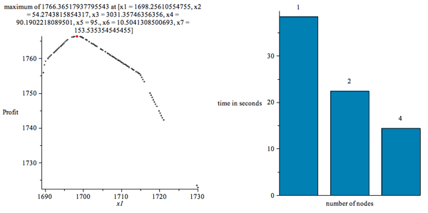
The chart shows the speedup for running this example on an Intel Core 2 Quad Q8200, with varying numbers of execution nodes. In addition to giving a nice speedup, this example also shows how easy it can be to convert a sequential program into a parallel one and get results in a fraction of the time.
This is a simple example that builds up a list with each node's number in it.
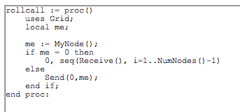
Run this program using the Launch command.

The numnodes option can be omitted. It is used here to generate a meaningful result even on computers with one or two cores. Note also that the results come back as soon as a node is finished, not in any particular order. Execution of the procedure in each of the external processes is truly concurrent. Due to multi-core technology, each process can execute at the same time. If you have 8 cores, the operation will take 1/8th of the time compared to the process running in serial.
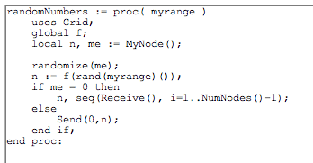
After the computation has been started, Send and Receive can be used for passing chunks of data to each individual node.
![]()
Above, the range, 1..10, is passed as an argument to the execution of randomNumbers on each node. The custom function, f, is not defined so it returns unevaluated. You can set a value for f, and use the 'imports' option to pass that value to all of the nodes.

Example 4: Monte Carlo Integration
Random values of x can be used to compute an approximation of a definite integral according to the following formula.

This example uses the multi-process execution functionality in order to evaluate the sum in parallel. See here for full details and source code
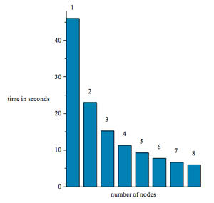
The chart shows that execution time drops from 46s to just 6s when we execute across 8 parallel nodes.
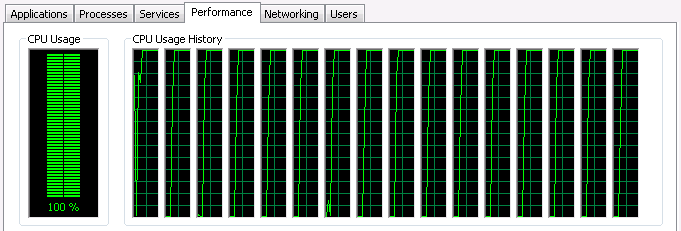
The screenshot at the top of this page is a view of Window's Task Manager showing CPU utilization when using 16 nodes, which includes processing on 8 real cores plus 8 virtual hyperthreads. It's nice to see all those CPUs being fully utilized.


