Optimization - Maple Features - Maplesoft

Maple

Single User Licenses
Multi-User Licenses
Upgrade
What's New  |  Features  |  Online Demos  |  Compare  |  Training  |  Community  |  Free Trial  |  Buy Maple
Optimization


Maple provides a collection of commands for numerically solving optimization problems, which involve finding the minimum or maximum of an objective function, possibly subject to constraints. The Optimization package enables you to solve linear programs (LPs), quadratic programs (QPs), nonlinear programs (NLPs), and both linear and nonlinear least-squares problems. Both constrained and unconstrained problems are accepted, and the package accepts a wide range of input formats.

You can also use Maple to perform global optimization. For more details, see Maple Global Optimization Toolbox.

Examples


Solving Linear Programs

Problem Description

Assume a problem where you want to:

Maximize the function `+`(x, y)

Subject to:


Solution

First, define the objective function:
ObjectiveFunctionLP1 := `+`(x, y)

`+`(x, y)

Then define a set containing all the constraint equations:

ConstraintEquationsLP1 := {`>=`(`+`(x, `*`(2, `*`(y))), 2), `>=`(`+`(`*`(4, `*`(x)), `-`(y)), 0), `<=`(x, 4), `<=`(y, 6.5), `<=`(`+`(x, `-`(y)), 2)}

{`<=`(0, `+`(`*`(4, `*`(x)), `-`(y))), `<=`(2, `+`(x, `*`(2, `*`(y)))), `<=`(x, 4), `<=`(y, 6.5), `<=`(`+`(x, `-`(y)), 2)}

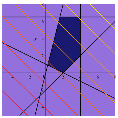
For a two-dimensional linear program, you can easily graph the feasible region, shown in blue below. The black lines indicate the constraints, and the red lines indicate the contours of the objective function `+`(x, y).

p1 := plots[inequal](ConstraintEquationsLP1, x = -5 .. 8, y = -5 .. 8, thickness = 2, optionsexcluded = (color =

p2 := plots[contourplot](ObjectiveFunctionLP1, x = -5 .. 8, y = -5 .. 8, thickness = 2); -1

plots[display](p1, p2)

Plot_2d

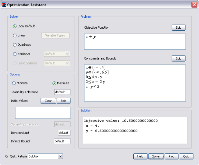
Using the Maximize command, find the solution that maximizes the objective function subject to the constraint equations. The first entry returned, 10.5, is the objective value at the optimal solution, while the second entry refers to a point, (4, 6.5), which is a solution point to the optimization problem. The point (4, 6.5) lies at the upper-right vertex of the feasible region.

Maximize(ObjectiveFunctionLP1, ConstraintEquationsLP1)

[10.5000000000000, [x = 4., y = 6.50000000000000000]]

This problem can also be solved using the interactive Optimization Assistant.

Image


Solving Non-Linear Programs

Problem Description

Find the point on the circle formed by the intersection of the unit sphere with the plane `+`(x, y, z) = `/`(1, 2) that is closest to the point (1, 2, 3).

Solution

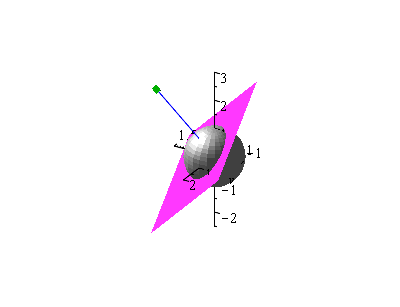
This problem can be easily conceptualized by plotting the unit sphere and the equation defining the intersecting plane.

p1 := plottools[sphere]([0, 0, 0], 1, color =

Plot_2d

The objective function is the squared distance between a point (x, y, z) and the point (1, 2, 3).

ObjectiveFunctionNLP1 := `+`(`*`(`^`(`+`(x, `-`(1)), 2)), `*`(`^`(`+`(y, `-`(2)), 2)), `*`(`^`(`+`(z, `-`(3)), 2)))

`+`(`*`(`^`(`+`(x, `-`(1)), 2)), `*`(`^`(`+`(y, `-`(2)), 2)), `*`(`^`(`+`(z, `-`(3)), 2)))

The point (x, y, z) is constrained to lie on both the unit sphere and the given plane. Thus, the constraints are:

ConstraintsEquationsNLP1 := {`+`(x, y, z) = `/`(1, 2), `+`(`*`(`^`(x, 2)), `*`(`^`(y, 2)), `*`(`^`(z, 2))) = 1}

{`+`(x, y, z) = `/`(1, 2), `+`(`*`(`^`(x, 2)), `*`(`^`(y, 2)), `*`(`^`(z, 2))) = 1}

You can minimize the objective function subject to the constraints using the NLPSolve command.

sol := NLPSolve(ObjectiveFunctionNLP1, ConstraintsEquationsNLP1)

[10.2919871984546809, [x = -.510336533719663588, y = .166666666666666492, z = .843669867052996847]]

Thus, the minimum distance is 10.29, and the closest point is (-0.51, 0.17, 0.84).


Solving Quadratic Programs

Problem Description

The Markowitz model is an optimization model for balancing the return and risk of a portfolio. The decision variables are the amounts invested in each asset. The objective is to minimize the variance of the portfolio's total return, subject to the following constraints: (1) the expected growth of the portfolio is at least some target level, and (2) the investment should not be more than the capital.

Solution

Let:

x[1] .. x[n] be the amounts you buy

c the amount of capital you have

R the random vector of asset returns over some period

r the expected value of R

G the minimum growth you hope to obtain

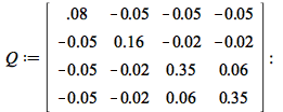
Q the covariance matrix of R

The objective function is Var(Sum(`*`(x[i], `*`(R[i])), i = 1 .. n)), which can be shown to be equal to `*`(`^`(x, T), `*`(Q, `*`(x))).

If, for example, n = 4, you would try to:

Minimize the function `*`(`^`(x, T), `*`(Q, `*`(x)))

Subject to:


Suppose you have the following data.

n := 4; -1

X := `<,>`(seq(x[i], i = 1 .. n)); -1

c := 10000; -1

G := 1000; -1

r := `<,>`(0.5e-1, -.20, .15, .30); -1

Q := Matrix(%id = 18446744078382340686); -1

This is a quadratic function of X, and so the quadratic programming can be used to solve the problem.

ObjectiveFunctionQP := expand(Typesetting:-delayDotProduct(Typesetting:-delayDotProduct(LinearAlgebra[Transpose](X), Q), X))

`+`(`*`(0.8e-1, `*`(`^`(x[1], 2))), `-`(`*`(.10, `*`(x[1], `*`(x[2])))), `-`(`*`(.10, `*`(x[1], `*`(x[3])))), `-`(`*`(.10, `*`(x[1], `*`(x[4])))), `*`(.16, `*`(`^`(x[2], 2))), `-`(`*`(0.4e-1, `*`(x[2]...

ConstraintEquationsQP := {`>=`(`+`(`*`(r[1], `*`(x[1])), `*`(r[2], `*`(x[2])), `*`(r[3], `*`(x[3])), `*`(r[4], `*`(x[4]))), G), `<=`(`+`(x[1], x[2], x[3], x[4]), c)}

{`<=`(1000, `+`(`*`(0.5e-1, `*`(x[1])), `-`(`*`(.20, `*`(x[2]))), `*`(.15, `*`(x[3])), `*`(.30, `*`(x[4])))), `<=`(`+`(x[1], x[2], x[3], x[4]), 10000)}

QPSolve(ObjectiveFunctionQP, ConstraintEquationsQP, assume = nonnegative)

[2232313.44316766, [x[1] = 3452.85892288522746, x[2] = 0., x[3] = 1068.80797452582034, x[4] = 2223.45285892288576]]

Thus, the minimum variance portfolio that earns an expected return of at least 10% is x[1] = 3452, x[2] = 0, x[3] = 1068, x[4] = 2223. Asset 2 gets nothing because its expected return is -20% and its covariance with the other assets is not sufficiently negative for it to bring any diversification benefits.


Solving Least-Square Problems

Problem Description

Neural networks are machine-learning programs that can learn to approximate functions using a set of sample function values called training data. To generate an output, a neural network applies a smooth function (typically, sigmoidal or hyperbolic tangent) to a linear weighting of the input data. To train the network, one assigns these weights so as to minimize the sum of squared differences between the desired and generated outputs over all data points in the training set. This is an optimization problem that can often be solved by least-squares techniques.

Solution

Assume that you have a sample training data set with five points. The first element of each point is the input, the second is the desired output.

x := [[1, 1], [.7, -1], [.1, -1], [.5, 1], [-.8, 1]]

[[1, 1], [.7, -1], [.1, -1], [.5, 1], [-.8, 1]]

Suppose that for a given input value x, the network outputs tanh(`+`(`*`(x, `*`(w[2])), w[1])), where w[1] and w[2] are the weights that are to be set. The residuals are the differences between these outputs and the desired outputs given in the training set:

Residual := seq(`+`(x[i][2], `-`(tanh(`+`(`*`(w[2], `*`(x[i][1])), w[1])))), i = 1 .. 5)

`+`(1, `-`(tanh(`+`(w[2], w[1])))), `+`(`-`(1), `-`(tanh(`+`(`*`(.7, `*`(w[2])), w[1])))), `+`(`-`(1), `-`(tanh(`+`(`*`(.1, `*`(w[2])), w[1])))), `+`(1, `-`(tanh(`+`(`*`(.5, `*`(w[2])), w[1])))), `+`(...

You can extract elements of the list x; using the selection operation. Then, use seq to create a sequence.

The objective function is the sum of squares of the residuals:

ObjectiveFunctionLeastSquares := add(`*`(`^`(Residual[i], 2)), i = 1 .. 5)

`+`(`*`(`^`(`+`(1, `-`(tanh(`+`(w[2], w[1])))), 2)), `*`(`^`(`+`(`-`(1), `-`(tanh(`+`(`*`(.7, `*`(w[2])), w[1])))), 2)), `*`(`^`(`+`(`-`(1), `-`(tanh(`+`(`*`(.1, `*`(w[2])), w[1])))), 2)), `*`(`^`(`+`...

Now, solve the optimization problem with the LSSolve command. Note that you only have to pass Maple the list of residuals.

LSSolve([Residual])

[2.36675848172506, [w[1] = .251236401056941061, w[2] = -.174677175635026300]]

The weights needed to minimize the sum of squared differences between the desired and generated outputs for w[1] and w[2] are .25123 and .174677.

Additional Resources